Binh and Korn
Description:
Optimization (min)
Multi-objective (2)
Constraints (2)
The general problem statement is given by:
\[\begin{split}\begin{cases} f_{1}\left(x,y\right) = 4x^{2} + 4y^{2} \\ f_{2}\left(x,y\right) = \left(x - 5\right)^{2} + \left(y - 5\right)^{2} \\ \end{cases}\end{split}\]
subject to:
\[\begin{split}\begin{cases} C_{1}\left(x,y\right) = \left(x - 5\right)^{2} + y^{2} \leq 25, \\ C_{2}\left(x,y\right) = \left(x - 8\right)^{2} + \left(y + 3\right)^{2} \geq 7.7 \\ \end{cases}\end{split}\]
where: \(-15\le x \le 30\) and \(-15\le y \le 30\).
The Pareto-optimal solutions are constituted by solutions: \(x=y \in [0.0, 3.0]\) and \(x \in [3.0, 5.0], y=3.0.\)
Step 1: Import python libraries and StarPSO classes
import numpy as np
from functools import lru_cache
from matplotlib import pyplot as plt
from star_pso.population.swarm import Swarm
from star_pso.population.particle import Particle
from star_pso.engines.standard_pso import StandardPSO
from star_pso.utils.auxiliary import pareto_front, cost_function
Step 2: Define the objective function
# Auxiliary method that returns a random value in [0, 1].
@lru_cache(maxsize=1024)
def random_weight(i: int = 0) -> float:
    return np.random.random()

# Multi-objective cost function.
@cost_function(minimize=True)
def fun_binh_korn(vector_xy: np.ndarray, **kwargs) -> float:

    # Set the penalty coefficient.
    rho = 5.0

    # Extract the values from the particle position.
    x, y = vector_xy

    # Compute each objective function.
    f1 = 4.0 * (x**2 + y**2)
    f2 = (x - 5.0)**2 + (y - 5.0)**2

    # Compute the constraints.
    C1 = max(0.0, (x - 5.0)**2 + y**2 - 25.0)**2
    C2 = min(0.0, (x - 8.0)**2 + (y + 3.0)**2 - 7.7)**2

    # Assign the weights.
    w1 = random_weight(kwargs["it"])
    w2 = 1.0 - w1

    # Compute the final value.
    f_value = w1*f1 + w2*f2 + rho*(C1 + C2)

    # Return the solution.
    return f_value
Step 3: Set the PSO parameters
# Set a seed for reproducible initial population.
SEED = 1821

# Random number generator.
rng = np.random.default_rng(SEED)

# Define the number of optimizing variables.
n_dim = 2

# Define the number of particles.
n_pop = 100

# Draw random samples for the initial points.
X_t0 = rng.uniform(-15.0, 30.0, size=(n_pop, n_dim))

# Initial population.
swarm_t0 = Swarm([Particle(x) for x in X_t0])

# Create a StandardPSO object that will perform the optimization.
test_PSO = StandardPSO(initial_swarm = swarm_t0,
                       obj_func = fun_binh_korn,
                       x_min = -15.0, x_max = 30.0)
Step 4: Run the optimization
test_PSO.run(max_it = 1500,
             options = {"w0": 0.70, "c1": 1.50, "c2": 1.50, "mode": "g_best"},
             reset_swarm = False, verbose = False, adapt_params = False)
Step 5: Extract the data for analysis and plotting
# Get the optimal solution from the PSO.
_, _, z_opt = test_PSO.get_optimal_values()

# Extract the optimal optimization variables.
x, y = z_opt

# Compute the final objective functions.
f1_opt = 4.0 * (x**2 + y**2)
f2_opt = (x - 5.0)**2 + (y - 5.0)**2

# Print the results.
print(f"x={x:.5f}, y={y:.5f}", end='\n\n')
print(f"f1(x, y) = {f1_opt:.5f}")
print(f"f2(x, y) = {f2_opt:.5f}")

# Stores the best positions.
best_n = []

for p in test_PSO.swarm.best_n(n_pop//2):
    # Extract the position.
    x_p, y_p = p.best_position

    # Compute the final objective functions.
    best_n.append((4.0*(x_p**2 + y_p**2),
                  (x_p - 5.0)**2 + (y_p - 5.0)**2))

# Convert to numpy.
best_n = np.array(best_n)
Step 6: Compute the Pareto front
# Create a list that will hold points that satisfy both constraints.
points = []

# Generate a 2D grid sample on [-15.0, 30].
for x in np.linspace(-15.0, 30.0, 100):

    for y in np.linspace(-15.0, 30.0, 100):

        # Compute the constraints.
        C1 = (x - 5.0)**2 + y**2 <= 25.0
        C2 = (x - 8.0)**2 + (y + 3.0)**2 >= 7.7

        # If both constraints are satisfied.
        if C1 and C2:

            # Evaluate both functions.
            f1 = 4.0 * (x**2 + y**2)
            f2 = (x - 5.0)**2 + (y - 5.0)**2

            # Keep the point in the list.
            points.append((f1, f2))
# _end_for_

# Convert lists to numpy.
points = np.array(points)

# Estimate the pareto front points.
pareto_points = pareto_front(points)
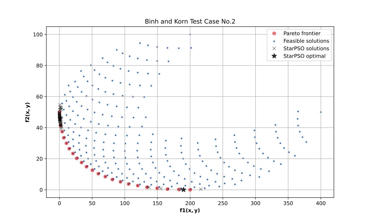
Step 7: Visualize the solutions
# Create a new figure.
plt.figure(figsize=(10, 6))

# Plot the Pareto front.
plt.plot(pareto_points[:, 0],
         pareto_points[:, 1],
         'ro', alpha=0.5, label="Pareto frontier")

# Plot all the feasible solutions.
plt.scatter(x=points[:, 0],
            y=points[:, 1],
            s=5, marker='o', label="Feasible solutions")

# Plot other points.
plt.plot(best_n[:, 0],
         best_n[:, 1],
         'kx', alpha=0.5, label="StarPSO solutions")

# Plot the optimal solution from the PSO.
plt.plot(f1_opt, f2_opt,
         'k*', markersize=10, alpha=0.8, label="StarPSO optimal")

# Tidy up the plot.
plt.title("Binh and Korn Test Case No.2")
plt.xlabel(r"$\mathbf{f1(x,y)}$")
plt.ylabel(r"$\mathbf{f2(x,y)}$")
plt.legend()
plt.grid(True)