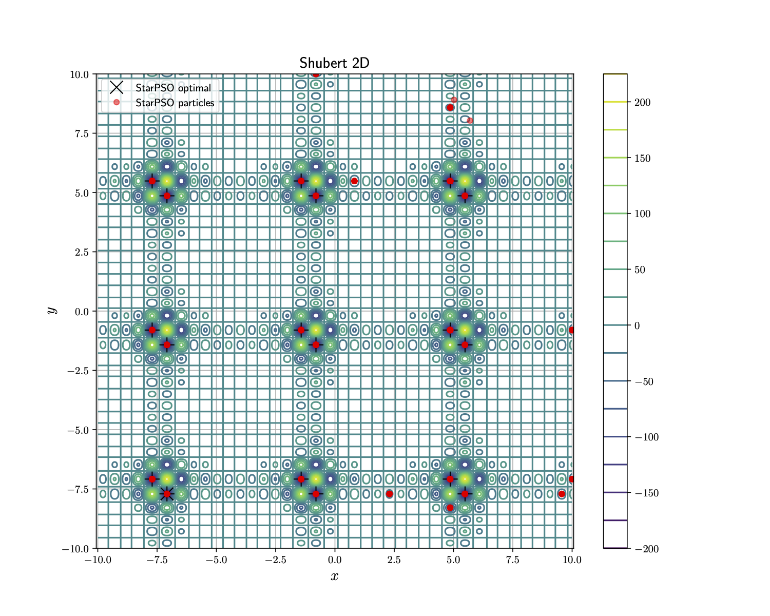
Shubert 2D
Description:
Optimization (min)
Multimodal (yes)
The Shubert function has several local minima and many global minima. The equation (for D=2) is given by:
\[f\left(x, y\right) = \left(\sum_{i=1}^5 i* \cos((i+1)*x + i)\right) \left(\sum_{i=1}^5 i* \cos((i+1)*y + i)\right)\]
The function is evaluated on the square \(x, y \in [-10, 10]\).
For D=2 the function has 18 global minima at \(f^*(x_{opt}, y_{opt}) = -186.7309\).
Step 1: Import python libraries and StarPSO classes
import numpy as np
from numba import njit
from matplotlib import pyplot as plt

# Enable LaTex in plotting.
plt.rcParams["text.usetex"] = True

from star_pso.population.swarm import Swarm
from star_pso.population.particle import Particle
from star_pso.engines.standard_pso import StandardPSO
from star_pso.utils.auxiliary import cost_function
Step 2: Define the objective function
# Auxiliary function.
@njit(fastmath=True)
def fun_shubert_vectorized(x: np.ndarray, y: np.ndarray) -> np.ndarray:
    # Define the range [1, 2, 3, 4, 5].
    i = np.arange(1, 6)

    # Calculate the first summation over each x.
    sum_x = np.sum(i[:, np.newaxis] * np.cos((i[:, np.newaxis] + 1) * x + i[:, np.newaxis]), axis=0)

    # Calculate the second summation over each y.
    sum_y = np.sum(i[:, np.newaxis] * np.cos((i[:, np.newaxis] + 1) * y + i[:, np.newaxis]), axis=0)

    # Return the product of both sums.
    return sum_x * sum_y

# Multimodal cost function.
@cost_function(minimize=True)
def fun_shubert2D(x_array: np.ndarray, **kwargs) -> float:
    # Extract the values.
    x, y = x_array

    # Compute the final value.
    f_xy = fun_shubert_vectorized(x, y)

    # Return the solution.
    return f_xy.item()
Step 3: Set the PSO parameters
# Set a seed for reproducible initial population.
SEED = 1821

# Random number generator.
rng = np.random.default_rng(SEED)

# Define the size of the problem (number of particles, dimensions).
n_pop, n_dim = 400, 2

# Set the bounds.
l_bounds = [-10.0, -10.0]
u_bounds = [+10.0, +10.0]

# Draw random samples for the initial points.
Xt0 = rng.uniform(-10.0, +10.0, size=(n_pop, n_dim))

# Initial population.
swarm_t0 = Swarm([Particle(x) for x in Xt0])

# Create a StandardPSO object that will perform the optimization.
test_PSO = StandardPSO(initial_swarm = swarm_t0,
                       obj_func = fun_shubert2D,
                       x_min = l_bounds,
                       x_max = u_bounds)
Step 4: Run the optimization
test_PSO.run(max_it = 500,
             options = {"w0": 0.75, "c1": 1.50, "c2": 1.50, "mode": "multimodal"},
             reset_swarm = False, verbose = False, adapt_params = False)
Step 5: Extract the data for analysis and plotting
# Get the optimal solution from the PSO.
_, f_opt, x_opt = test_PSO.get_optimal_values()

# Print the results.
print(f"x={x_opt}, f(x) = {-f_opt:.5f}")

# Stores the best positions.
best_n = []

for p in test_PSO.swarm.best_n(n=n_pop):
    best_n.append(p.position)

best_n = np.unique(np.array(best_n), axis=0)

# Prepare a list with all the global optima.
global_optima =[(-7.0835, -7.7083),
                (-7.0835, -1.4250),
                (-7.0835, +4.8601),

                (-0.8003, -7.7083),
                (-0.8003, -1.4250),
                (-0.8003, +4.8601),

                (+5.4858, -7.7083),
                (+5.4858, -1.4250),
                (+5.4858, +4.8601),

                (-7.7083, -7.0835),
                (-7.7083, -0.8003),
                (-7.7083, +5.4858),

                (-1.4250, -7.0835),
                (-1.4250, -0.8003),
                (-1.4250, +5.4858),

                (+4.8601, -7.0835),
                (+4.8601, -0.8003),
                (+4.8601, +5.4858)]

optima = np.array(global_optima)
Step 6: Visualize the solutions
# Prepare the plot of the real density.
x, y = np.mgrid[-10.0:10.01:0.01, -10.0:10.01:0.01]

plt.subplots(figsize=(10, 8))

# First plot the contour of the "true" function.
plt.contour(x, y, np.reshape(fun_shubert_vectorized(x.flatten(),
                                                    y.flatten()),
                             shape=(x.shape[0], y.shape[0])),
            levels=15)

# Plot the global optima.
plt.plot(optima[:, 0], optima[:, 1], "k+", markersize=14)

# Plot the optimal PSO.
plt.plot(x_opt[0], x_opt[1], "kx", markersize=12, label="StarPSO optimal")

# Plot the best_n.
plt.plot(best_n[:, 0], best_n[:, 1], "ro", alpha=0.5, markersize=5, label="StarPSO particles")

# Add labels.
plt.xlabel("$x$", fontsize=14)
plt.ylabel("$y$", fontsize=14)
plt.title("Shubert 2D", fontsize=14)
plt.legend()

# Final setup.
plt.colorbar()
plt.axis("equal")
plt.grid()